In this note we analyse the SMEM layouts and examine how CUTLASS and Triton represent them. The non-swizzling cases need special handling and omitted for simplicity in this note. We also only talk about 16B atomicity swizzling for simplicity.

Core Matrix vs Swizzle Atom

Core Matrix

“Core matrix” is a deprecated term and no longer available in official documents. It used to be a term used to help define Leading Dimension Byte Offset (LBO) and Strided Dimension Byte Offset (SBO), which are two very important parameters required to supply SMEM layout representations to hardware such that Tensor Core knows where to find operands.

For example, in this Colfax tutorial,

Each core matrix has a strided direction and a contiguous direction, such that its length is 8 in the strided direction and 16 bytes in the contiguous direction. LBO (leading dimension byte offset): the distance, in bytes, between two adjacent core matrices in the K dimension. SBO (stride dimension byte offset): the distance, in bytes, between two adjacent core matrices in the M or N dimension.

which might be correct to that specific instance of MMA in the blog, but doesn’t cover MN-major cases.

As can be seen later in this note, the concept of core matrix is indeed no longer needed. And we only need Swizzle Atom to define SBO and LBO.

Swizzle Atom

As of Jun 2026, the official PTX documentation defines the SMEM layout with the concept of “Swizzle Atom”. A Swizzle Atom with s Bytes swizzling mode is a matrix of 8 * s Bytes where 8 is on the strided dimension (e.g. M/N dim for K-major) and s Bytes is on the leading dim.

All the elements in a Swizzle Atom are compactly stored in a segment of contiguous physical SMEM. The SMEM swizzling then wouldn’t “exchange” elements across two Swizzle Atom. It’s only inside one Swizzle Atom. Also note the basic unit of swizzling is 128 bits or 16 bytes (in 16B atomicity mode). No “exchange” happens inside a single unit.

SBO is then defined as the byte offset between two adjacent Swizzle Atoms on strided dim.

LBO is defined as the byte offset between two adjacent Swizzle Atoms on leading dim. Note for K-major LBO is ignored because it’s “not used, assumed to be 1” in PTX doc.

Triton

In Triton compiler there’s a function called getCoreMatrixLinearLayout. It’s in fact getting a Linear Layout tile of a Swizzle Atom despite the naming. Since Linear Layout incorporates swizzling, the output of this function already encodes the full swizzled layouts of such an Atom. e.g.

Full tensor shape: 128, 256
Layout encoding: #ttg.nvmma_shared<{swizzlingByteWidth = 128, transposed = false, elementBitWidth = 16}>
getCoreMatrixLinearLayout output: 
 - offset=1 -> (0, 1)
   offset=2 -> (0, 2)
   offset=4 -> (0, 4)
   offset=8 -> (0, 8)
   offset=16 -> (0, 16)
   offset=32 -> (0, 32)
   offset=64 -> (1, 8)
   offset=128 -> (2, 16)
   offset=256 -> (4, 32)
where out dims are: [dim0 (size 8), dim1 (size 64)]

SMEM Layouts for an MMA instruction

The PTX documentation records canonical CUTE layouts for the SMEM tensor of one single MMA instruction:

• T = 128 / sizeof-elements-in-bits T represents scale factor which normalizes matrix element types to 128-bits.
• m represents the number of repeating patterns across rows.
• k represents the number of repeating patterns across columns.

* As shown later in this note, the factor k in K-major layout is in fact not needed and should be dropped.

MN major

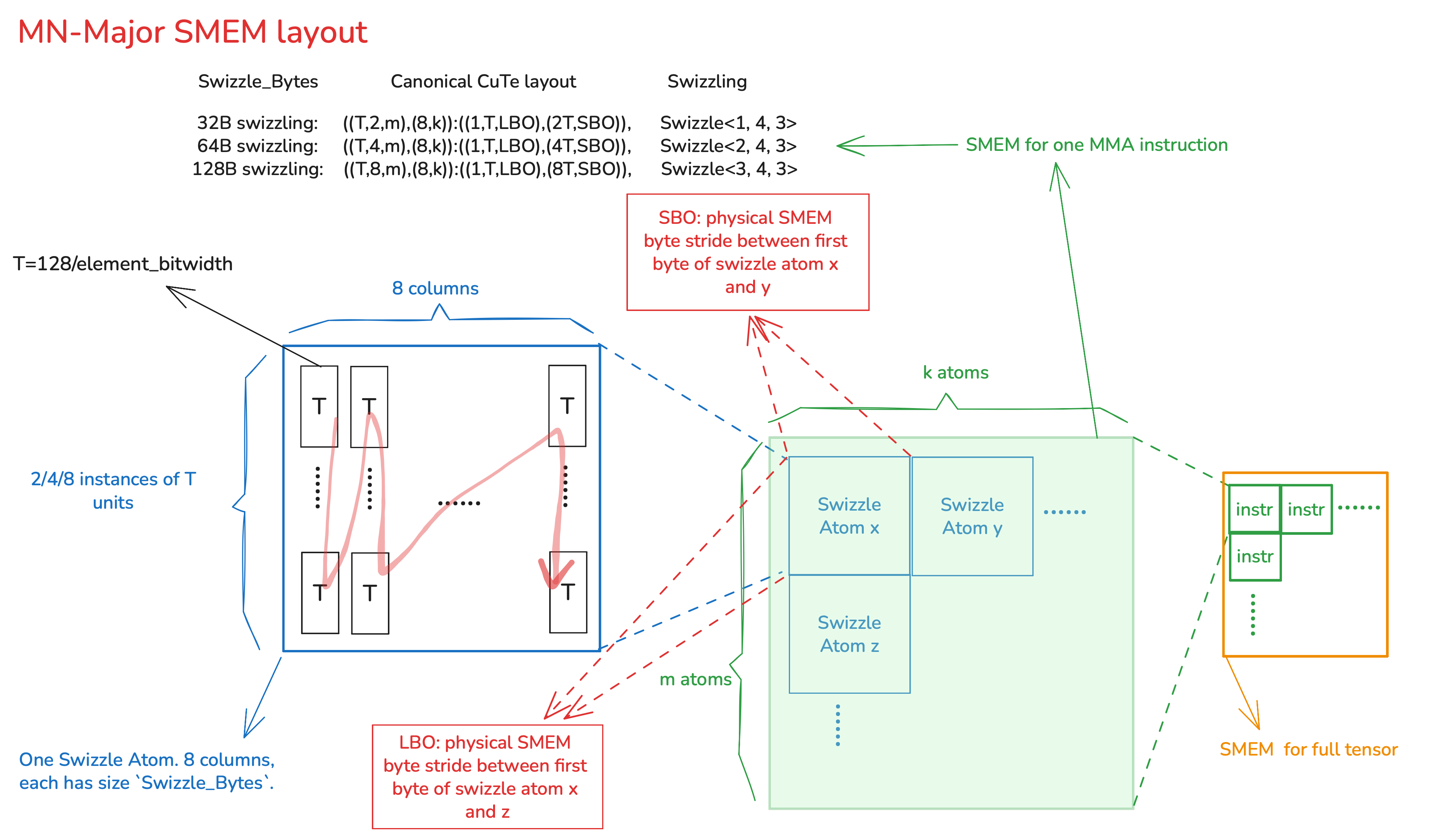
(The figure is drawn as M/N x K following CUTLASS convention)

The Canonical CuTe layout in PTX documentation is consistent with CUTLASS, and is shown in the figure.

Inside a Swizzle Atom, there’re 8 columns that’re adjacent to each other on physical memory. Each column is a contiguous segment on physical memory and has size equal to swizzling byte width.

It’s up to the user how to distribute the Swizzle Atoms(along MN or K dim first). As long as LBO and SBO are provided, the hardware knows where in the physical memory to look for desired Atoms. Note both LBO and SBO are needed because hardware needs to know where on the physical memory to load Swizzle Atom y, z and others.

From the getCoreMatrixLinearLayout function above, Triton always distributes the Atoms along strided dim first up to a TMA block.

K major

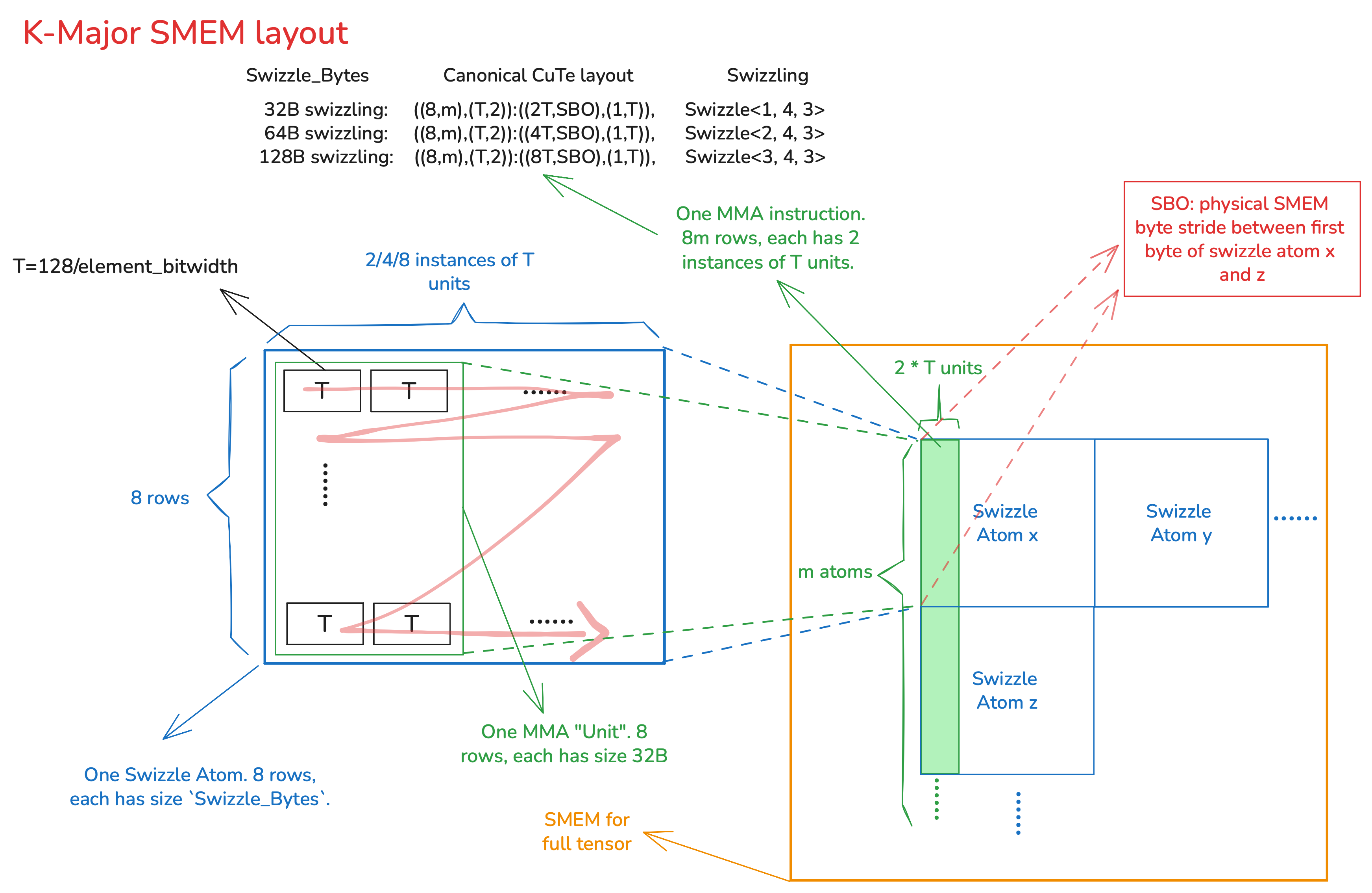
The Canonical CuTe layout in PTX documentation is different from CUTLASS in that CUTLASS dropped factor k. We adopt CUTLASS’s layouts as the source of truth with confirmation from Nvidia.

Inside a Swizzle Atom, there’re 8 rows adjacent to each other on physical memory. Each row is a contiguous segment on physical memory and has size equal to swizzling byte width.

It’s up to the user how to distribute the Swizzle Atoms(along MN or K dim first). For 64B/128B swizzling, an MMA “unit” SMEM is smaller than a Swizzle Atom and each row in a Swizzle Atom contains elements from 2/4 different MMA instructions. This is OK because swizzling just deterministically tells hardware the exact location of each element. e.g. For 128B swizzling this table shows where in the physical SMEM to find the 8*2 T units of the first MMA instruction:

Each MMA instruction’s SMEM operand spans across multiple Swizzle Atoms along MN dim, but only one (or partial) Atom along K dim. So given location of Atom x, the hardware needs SBO to know where to load Atom z and others along MN dim. However, LBO is not needed (except non-swizzling cases, not shown in the figure) because for example Atom y is not needed by the MMA instruction in the figure.

From the getCoreMatrixLinearLayout function above, Triton always distributes the Atoms along strided dim first up to a TMA block.

References

• PTX ISA Documentation v9.3
• Colfax CUTLASS Tutorial: Fast Matrix-Multiplication with WGMMA on NVIDIA® Hopper™ GPUs
• CUTLASS source code for SM100 UMMA descriptors
• Triton source code for NVMMAShared encoding to Linear Layout conversion

Special thanks to Bingyi Zhang from Nvidia! A great amount of details and nuances in this note came from extensive discussions and collaborations with Bingyi.

In this short note, we derive the backward gradient of a matrix multiplication with minimal math background.

Forward Pass

Matrix shapes:

Meaning of dY

In backward prop, we are given the input that has known values and the same shape as $Y$:

where $L$ is a scalar loss.

Thus:

Intuitively, $dY[i][j]$ measures how much the loss $L$ changes if $Y[i][j]$ increases slightly.

for a very small $h$.

Goal

We want to compute

Each element

represents how much the loss changes if $X[i][j]$ increases.

Chain Rule

To compute a single element $dX[i][j]$ in $dX$, we apply the chain rule through $Y$:

Note both $\frac{\partial L}{\partial Y}$ and $\frac{\partial Y}{\partial X[i][j]}$ are of the same shape as Y, and $dX[i][j]$ is the sum of pointwise product of them.

Also note element at index $[a][b]$ in $\frac{\partial Y}{\partial X[i][j]}$ is just $\frac{\partial Y[a][b]}{\partial X[i][j]}$.

Using the shorthand $dY[a][b] = \frac{\partial L}{\partial Y[a][b]}$:

Intuitively:

• $\frac{\partial Y[a][b]}{\partial X[i][j]}$ measures how $X[i][j]$ affects $Y[a][b]$
• $dY[a][b]$ measures how $Y[a][b]$ affects the loss $L$

Multiplying them gives the influence path

Summing over all $a,b$ aggregates all such paths, showing the influence $X[i][j]$ on $L$.

Expand the Forward Definition

From matrix multiplication:

That is:

Dependency Observation

If $b \ne j$, then $Y[a][b]$ does not depend on $X[i][j]$. It only depends on row $a$ of $W$ and column $b$ of $X$.

Therefore:

Thus only terms where $b = j$ contribute.

The formula simplifies from

to

Compute the Partial Derivative

Consider

The only term involving $X[i][j]$ is

Therefore

Then

becomes

then exchange position of two elements

Recognizing the Matrix Form

Notice

Thus

This is exactly the definition of matrix multiplication

Final Result

For the forward operation

the backward gradients are

If we go through a very similar process, we could also prove

How to remember this: for Y=WX or Y=XW, when we want to compute dX given dY, we always just swap positions of X(dX) and Y(dY), and then just transpose W without changing its location in the equation.

Forward Pass

Given a vector of attention scores $S \in \mathbb{R}^{N}$, softmax produces:

Note $P[i] > 0$ and $\sum_i P[i] = 1$.

In flash attention, softmax is applied independently to each row of the attention score matrix $S = QK^T$. Everything below applies per row.

Meaning of dP

In backward prop, we are given the input that has known values and the same shape as $P$:

where $L$ is a scalar loss. Each element:

measures how much the loss $L$ changes if $P[i]$ increases slightly.

Goal

We want to compute

Each element

represents how much the loss changes if $S[i]$ increases.

Chain Rule

To compute a single element $dS[i]$, we apply the chain rule through $P$:

Note both $\frac{\partial L}{\partial P}$ and $\frac{\partial P}{\partial S[i]}$ have the same shape as $P$, and $dS[i]$ is the sum of pointwise product of them.

Also note element at index $[j]$ in $\frac{\partial P}{\partial S[i]}$ is just $\frac{\partial P[j]}{\partial S[i]}$.

Note: unlike matmul, every $P[j]$ depends on $S[i]$ because $S[i]$ appears in the denominator $\sum_k e^{S[k]}$. So no terms drop out.

Compute the Partial Derivatives

We need $\frac{\partial P[j]}{\partial S[i]}$ for two cases.

Case 1: $j = i$

Using the quotient rule where the numerator is $e^{S[i]}$ and the denominator is $\sum_k e^{S[k]}$:

Case 2: $j \ne i$

Here the numerator $e^{S[j]}$ does not depend on $S[i]$, so using the quotient rule:

Substitute Back

Split the chain rule sum into the $j = i$ term and the $j \ne i$ terms:

Factor out $P[i]$:

Expand the first term:

Notice that $dP[i] \cdot P[i] + \sum_{j \ne i} dP[j] \cdot P[j] = \sum_{j} dP[j] \cdot P[j]$, so:

Define the dot product as a single scalar:

So:

Note $D$ is a fixed scalar no matter what value $i$ is.

Final Result

For the forward operation

the backward gradient is

where

Or in vector form:

where $\odot$ is elementwise multiplication and $D$ is a scalar (per row).

Why This Matters for Flash Attention

In flash attention, softmax is applied row-wise to the attention score matrix $S = QK^T$, and the backward pass must be computed without materializing the full attention matrix in HBM.

The formula $dS = P \odot (dP - D)$ is perfectly suited for this because:

1. $D$ is just a scalar per row. By definition:

This looks like it needs both $dP$ and $P$, which are full-sized attention matrices we want to avoid materializing. But recall the forward output of attention is $O = PV$, and its gradient is $dO$. We have $dP = dO \cdot V^T$, so:

Swapping the order of summation:

since $\sum_j P[i][j] \cdot V[j][l] = O[i][l]$ by the forward definition $O = PV$. So:

This is just a row-wise dot product of $dO$ and $O$ — both of which are already available in HBM from the forward pass and the incoming gradient. No need to recompute $P$ or $dP$ for this step.

1. Recomputing $P$ per tile using saved row sum. During the forward pass, we never have a full row of true $P$ values at once — each tile only sees a partial denominator. But the forward pass saves the sum of exponentials per row:

In the backward pass, for a tile covering column block $j$, we recompute the local attention scores $S[i][j] = Q[i] \cdot K[j]^T$ and recover the true softmax values for that tile:

This is exactly the softmax definition. The key insight is that $L[i]$ encodes the full-row denominator, so any tile can produce its correct $P$ values independently.

1. Each tile is independent. With $D$ precomputed (step 1) and $P$ recoverable per tile (step 2), we form $dP$ from $dO$ and $V^T$ for that tile, and apply $P \odot (dP - D)$. The subtraction of $D$ is the only term that couples different columns within a row, and since $D$ is already a known scalar, each tile can be processed independently.